Continuation from the previous 41 parts, starting from https://www.nikoport.com/2013/07/05/clustered-columnstore-indexes-part-1-intro/
Important Disclaimer – I have started writing this blog post over 1 months ago, but because of all engagements such as SQLSaturday Portugal, only today at night managed to finally finish it.
Big thanks go to Chris Adkin for very interesting ideas exchange, if you want a deep stuff on query processing – roll over to his blog.
This time I decide to dedicate a whole blog post into the matter of Materialisation, the concept which exists in SQL Server since 2005 Service Pack 2 version and applies universally to Columnstore as well as to the traditional Rowstore.
I consider that a good understanding of Materialisation Strategies might provide a better understanding of Columnstore Indexes functioning and their performance optimisations.
Materialisation:
Materialisation is the process of transforming encoded data into human readable tuples.
SQL Server 2008 has introduced 2 types of row compression – Page & Row that allowed to optimise storage space by using compression algorithms.
But even before that the VarDecimal compression included in SQL Server 2005 SP2 is a type of storage optimisation that allowed to save space by not using the additional bits & bytes defined for 2 of the standard types – Decimal and Numeric.
Since Columnstore Indexes are implemented by using different types of compression, every time we store some data we need to dematerialise(compress) data before storing it, and if we are to access some of the stored data – we need to materialise(decompress) it.
Consider a simple table with just one column, containing a name of a person:
 This table contains 12 tuples with 6 distinct values – it is a very simple case. Let us compress this table with the most simple of Dictionary compressions in order to be able to emulate the materialisation strategies. The process of encoding the original values into compressed ones is materialisation or compression.
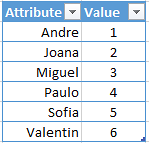 On the right side you can see the dictionary that was created in order to achieve the compression – we have exactly 6 distinct values for our Dictionary where each of them receives an integer number (Notice that I am simplifying everything greatly in order to come through with a more simple case).
The values can be sorted or unsorted, it will ultimately depend on the actual design implementation.
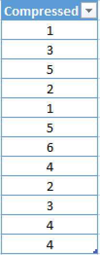
Now our attribute vector shall look this way whenever we process it and in order to get any meaning out of those numbers we shall need to combine it with our Dictionary.
So for example if we want to execute the statement “Select Name from dbo.SampleTable where Name = ‘Andre’;” the execution process will have to read the data from the Dictionary, finding out if there is an entry that has a label equal to ‘Andre’ and then to read the value assigned to this entry, which in our case is equal to 1.
Next phase would be to scan our Compressed Table and to find out the rows containing value 1 which will be then decompressed and returned to the user. This makes more sense whenever we have other columns in our table which will be simply read and joined with the identified rows.
Materialisation Types:
Materialisation can be parallel and pipelined – both of these methods have their advantages and disadvantages. Parallel Materialisation consumes more memory while delivering the best performance, while Pipelined Materialisation has lower performance while consuming less resources at a time.
There are 2 principal strategies related to the execution time of the materialisation: Early Materialisation & Late Materialisation.
Early Materialisation:
This concept focuses on all necessary column retrieval in the early stages of the query execution. The idea is to decompress the encoded values as soon as possible, thus creating a row which can be processed and worked on in the later stages of query execution.
There is a number of clear disadvantages of using Early Materialisation, such as
– Construction of all involved tuples. This means that we shall need to decompress all of the columns by themselves, and then glue them together. Only basic segment elimination shall be applied before the decompression.
– Very extensive memory utilisation. All decompressed information might spend a significant memory bandwidth for storing and working with your decompressed tuple information.
At all, I do not know any of the advantages for the Early Materialisation. This type of materialisation is happening mostly on the basic systems without good Query Optimiser or because the query itself requires tuples to be materialised on the earlier stages – for example if we executing some type of an operation that can’t be done on the compressed data – such as a complex text search.
So now you are wondering, how can I ensure Later Materialisation?
Leave it to Query Optimiser, it will do the best job possible in this situation, if possible, shifting materialisation to a later stage.
Late Materialisation:
Late Materialisation is the concept that focuses on delaying the materialisation (conversion of the compressed data into readable format) for projecting columns as much as possible until one of the latest stages of the query execution, thus enabling less amounts data to travel between iterators.
In a perfect situation the materialisation takes place at the very last moment – before presenting results to the user.
This is rather difficult task and a lot of times quite impossible, for example if we are joining tables on the columns compressed with different compression algorithms or containing different dictionaries.
On our sample table, execute the following query and consider what is going to happen – stage by stage:
select name, count(*)
    from dbo.SampleTable
    group by name
    order by count(*) desc;
First we shall have to scan the content of our sample table with names entirely.
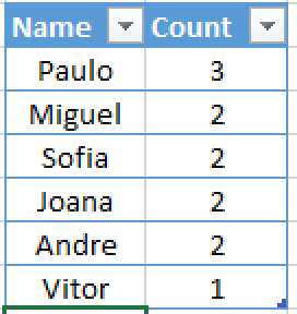
Secondly we shall group the distinct values together and our intermediate results should look like this:
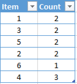 Notice that we have all the distinct values for the names in the order how we have found them in the original. This might look different if we would be using parallel access and reading from this table.
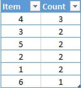 Next step is ordering the table, and so we sort the found counts according to the original SELECT statement. Now we have our result completely calculated and the only thing that is missing is to convert the results into humanly readable form by decompressing them.
 In the final step we are materialising(decompressing) the results into something that user can understand. This way we have actually executed all operations on compressed values thus delaying decompression process – having this way obtained Late Materialisation.
The major advantage here are the memory bandwidth for processing the query as well as the Batch Mode L2 cache operations.
Occupied memory bandwidth will be significantly lower in the case of compressed values enabling processing more queries in parallel and for the Batch Mode operations we can fit more data into our L2 cache this way enabling to reach the maximum allowed number of rows per batch – 900.
Sample Table on SQL Server 2014
Talking about the benefits of Late Materialisation, consider a simple query on a compressed table for real:
 Here we have 4 columns with 5 tuples and not so much different information consisting of a 3 integer & 1 variable character column. Let us imagine some simple type of compressions, without any complex binary additions that Columnstore Indexes enjoy in SQL Server, which would naturally improve the compression rate on the big tables in DatawareHouses and BI Solutions.
 On the picture at the right side, you can the results of some simple compressions that I have applied on the table. As a result we have made our table 36% of the size of the original, thus compressing almost 3 times the amount of information. That is almost like 3 times, which is a nice improvement given in fact that I want to run a couple of analytical queries on my table.
Let’s try to find out the total sales per each of our sales managers:
select SalesManager, sum(SalesAmount) as ManagerSales
from dbo.SampleTable
group by SalesManager
option (maxdop 1);
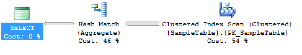 In our sample single threaded execution plan (generated with a help of MAXDOP = 1 for more simplicity) we have 3 simple iterators – Select, Hash Match (Aggregate) and a Clustered Index Scan (this is a Row Store).
The difference between Early & Late Materialisation here would be decompressing following:
– for Early Materialisation we would decompress right after reading data, at Clustered Index Scan operator;
– for Late Materialisation we would try to decompress as late as possible, in a perfect world at the Select Statement, way after all possible & executable operations are done;
In a row store we are reading our 118 bytes from the storage and transferring them to the Hash Match iterator, grouping data by SalesManager and then delivering a couple of grouped rows back to the user.
This is a good example of an early materialisation, since we are materialising the tuples right after reading them from the disk.
Compressed Table
Imagine that we do that on the compressed table, reading the data from the disk, decompressing all the data on the reading operation (Clustered Index Scan) and delivering the full 118 bytes to the Hash Match iterator – this is still the early materialisation, since we have materialised (decompressed) our tuples on the earliest opportunity.
In the case of Late Materialisation in Columnstore Indexes we would read only the needed columns SalesManager & SalesAmount (25+10) 35 bytes instead of 118 bytes, without applying decompression strategy.
On the second step I would apply Hash Match operation on the compressed column and since I have applied dictionary & bit vector compressions on the SalesManager column – I would need to work with just with 3 bytes, because I do not care yet about the real value behind the aggregation – I simply want to aggregate on some distinct values.
We shall have to sum the totals of the SalesAmount here, this operation can be performed on the compressed data as well, thus we are constantly improving the memory bandwidth as well as the performance of our query execution.
On the last 3rd iterator we shall simply need to materialise (decompress) the aggregated information, enabling the correct visualisation to the user, and once again the information has been passed between 2nd and 3rd iterators still compressed.
We shall suffer a penalty on the last step because of the spent CPU cycles to decompress the information, but in a typical situation it is quite irrelevant to the total duration of the query, especially in the analytical queries where we have to decompress just a couple of rows.
This is just a simple example, but imagine we are dealing not with the bytes but with GB or TB of information :)
The good, The bad & the Ugly
You might think, this is all fine – but what about more practical examples with more data?
Let’s use a freshly restored copy of ContosoRetailDW database, drop primary & foreign keys from FactOnlineSales and create Clustered Columnstore Index:
USE [master]

alter database ContosoRetailDW
	set SINGLE_USER WITH ROLLBACK IMMEDIATE;

RESTORE DATABASE [ContosoRetailDW]
	FROM  DISK = N'C:\Install\ContosoRetailDW.bak' WITH  FILE = 1,
		MOVE N'ContosoRetailDW2.0' TO N'C:\Data\ContosoRetailDW.mdf',
		MOVE N'ContosoRetailDW2.0_log' TO N'C:\Data\ContosoRetailDW.ldf',
		NOUNLOAD,  STATS = 5;

alter database ContosoRetailDW
	set MULTI_USER;
GO

ALTER DATABASE [ContosoRetailDW] SET COMPATIBILITY_LEVEL = 120
GO
use ContosoRetailDW;

alter table dbo.[FactOnlineSales] DROP CONSTRAINT PK_FactOnlineSales_SalesKey

alter table dbo.[FactOnlineSales] DROP CONSTRAINT FK_FactOnlineSales_DimCurrency
alter table dbo.[FactOnlineSales] DROP CONSTRAINT FK_FactOnlineSales_DimCustomer
alter table dbo.[FactOnlineSales] DROP CONSTRAINT FK_FactOnlineSales_DimDate
alter table dbo.[FactOnlineSales] DROP CONSTRAINT FK_FactOnlineSales_DimProduct
alter table dbo.[FactOnlineSales] DROP CONSTRAINT FK_FactOnlineSales_DimPromotion
alter table dbo.[FactOnlineSales] DROP CONSTRAINT FK_FactOnlineSales_DimStore
GO

Create Clustered Columnstore Index PK_FactOnlineSales on dbo.FactOnlineSales;
Now, for testing, let’s create an ordered copy of FactOnlineSales table, using for this purpose the Segment Clustering technic (Notice that I am sorting on the ProductKey column):
SELECT [OnlineSalesKey]
      ,[DateKey]
      ,[StoreKey]
      ,[ProductKey]
      ,[PromotionKey]
      ,[CurrencyKey]
      ,[CustomerKey]
      ,[SalesOrderNumber]
      ,[SalesOrderLineNumber]
      ,[SalesQuantity]
      ,[SalesAmount]
      ,[ReturnQuantity]
      ,[ReturnAmount]
      ,[DiscountQuantity]
      ,[DiscountAmount]
      ,[TotalCost]
      ,[UnitCost]
      ,[UnitPrice]
      ,[ETLLoadID]
      ,[LoadDate]
      ,[UpdateDate]
  into dbo.FactOnlineSalesOrdered
  FROM [dbo].[FactOnlineSales];

create clustered index PK_FactOnlineSalesOrdered
	on dbo.FactOnlineSalesOrdered (ProductKey);

create clustered columnstore index PK_FactOnlineSalesOrdered
	on dbo.FactOnlineSalesOrdered
	with (drop_existing = on, maxdop = 1);
Let’s run a simple query on the our test tables:
select  prod.ProductName, min(CustomerKey), max(CustomerKey), max(OnlineSalesKey), sum(sales.SalesAmount) as Sales
	from dbo.FactOnlineSales sales
		inner join dbo.DimProduct prod
			on sales.ProductKey = prod.ProductKey
	group by prod.ProductName;

select  prod.ProductName, min(CustomerKey), max(CustomerKey), max(OnlineSalesKey), sum(sales.SalesAmount) as Sales
	from dbo.FactOnlineSalesOrdered sales
		inner join dbo.DimProduct prod
			on sales.ProductKey = prod.ProductKey
	group by prod.ProductName;
Let’s look at the execution plans:
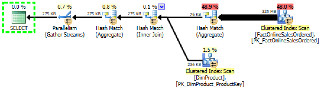
Both execution plans looks almost completely equal besides that on the first query, for unsorted table, the percentages for the Hash Match Aggregate is 49.2%(here 48.9%) and Clustered Columnstore Index Scan 47.7%(here 48.0%), but there is a significant difference hidden below those pretty arrows and numbers. Performance. Execution Time. Resources.
Take a look at the execution times:

Yes, your eyes are not lying – 352 milliseconds vs 222 milliseconds total execution time and the CPU resources 578 ms vs 437 ms.
Over 100 ms differences which represents over 35% improvement and the CPU resources gives over 140 ms and 25% improvement.
Amazing, but how ???
2 Words – Late Materialisation.
Take a good look at the execution plan on the image above – do you see 325MB of data flowing from the FactOnlineSalesOrdered Clustered Columnstore Index Scan to Hash Match Aggregate? Are they real or are they simply estimate numbers?
Let us see the whole size of the respective tables:
exec sp_spaceused FactOnlineSales, true;
exec sp_spaceused FactOnlineSalesOrdered, true;

I swear that on my computer both tables are rounding 163MB, which makes sense, because I am using 2 cores on this VM (163MB times 2 might be approximated to 325 MB), so each core has scanned the whole Columnstore …
Wait a second!!!
With Clustered Columnstore Indexes we have segment elimination and in practice we read only those columns that our query includes, which means that those pure estimates are pointing directly to nowhere. :)
For now let’s leave the Dimension table and dive into Clustered Columnstore Index:
Let’s take a detailed look into the used columns and their segment sizes (no segment elimination is happening in our query as the query has no predicate):
select object_name(part.object_id) as TableName
	 ,seg.column_id as ColumnId
	 ,cols.name as ColumnName
	 ,sum(on_disk_size) as on_disk_size
	from sys.column_store_segments seg
		inner join sys.partitions part
			on seg.hobt_id = part.hobt_id
		inner join sys.columns cols
			on cols.object_id = part.object_id and cols.column_id = seg.column_id
	where part.object_id in (object_id('FactOnlineSales'), object_id('FactOnlineSalesOrdered') )
		and cols.name in ('CustomerKey','OnlineSalesKey','SalesAmount','ProductKey')
	group by part.object_id, cols.name, seg.column_id
	order by seg.column_id, object_name(part.object_id);
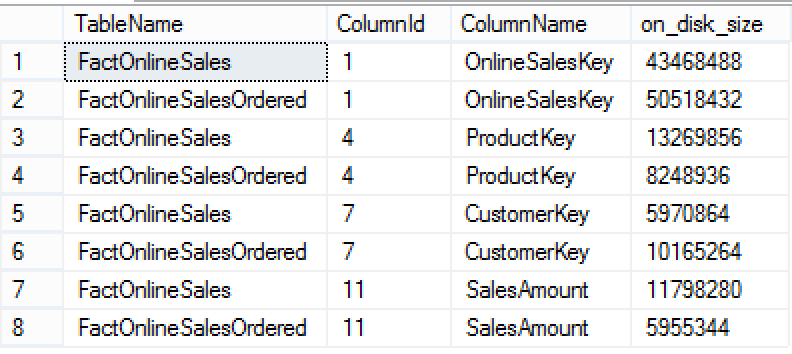
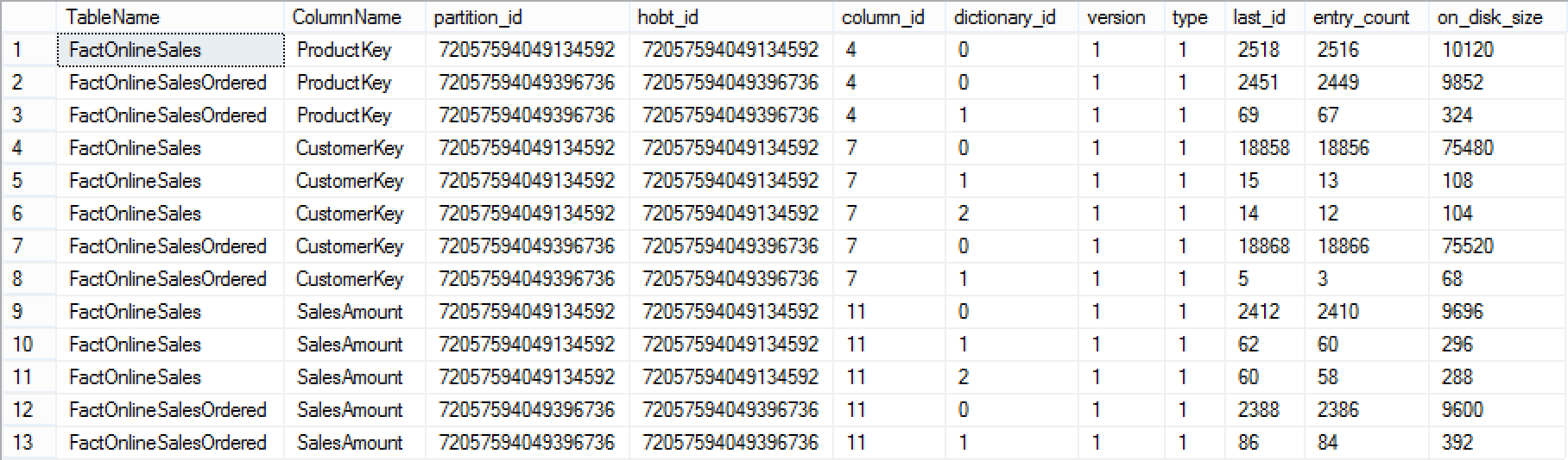
Notice that total compressed sizes of the same columns vary greatly, for the most important column – ProductKey we have a 13 MB vs 8 MB differences and for the column OnlineSalesKey the difference goes into opposite direction – the unsorted table has over 7 MB less than the sorted table – 50 MB vs 43MB. Notice that for the sizes involved those differences represent a very significant percentage.
Measuring the totality of the columns Segments involved we can see that the difference is not really significant:
select object_name(part.object_id) as TableName
	 ,sum(on_disk_size) as on_disk_size
	from sys.column_store_segments seg
		inner join sys.partitions part
			on seg.hobt_id = part.hobt_id
		inner join sys.columns cols
			on cols.object_id = part.object_id and cols.column_id = seg.column_id
	where part.object_id in (object_id('FactOnlineSales'), object_id('FactOnlineSalesOrdered') )
		and cols.name in ('CustomerKey','OnlineSalesKey','SalesAmount','ProductKey')
	group by part.object_id
	order by object_name(part.object_id);

Both sizes are around 74,5 MB.
What about dictionaries then:
select object_name(part.object_id) as TableName
	 ,cols.name as ColumnName
	 ,dict.*
	from sys.column_store_dictionaries dict
		inner join sys.partitions part
			on dict.hobt_id = part.hobt_id
		inner join sys.columns cols
			on cols.object_id = part.object_id and cols.column_id = dict.column_id
	where part.object_id in ( object_id('FactOnlineSales'), object_id('FactOnlineSalesOrdered'))
		and cols.name in ('CustomerKey','OnlineSalesKey','SalesAmount','ProductKey')
	order by cols.column_id, object_name(part.object_id);
The dictionaries look pretty similar even though this might be very deceiving, because compression dictionary size is 1 thing and its usage is a different story.
In any case we know our segments and know that the dictionaries are not 16 MB big and will not affect IO greatly in a direct way.
Memory Dive:
There are some very interesting little differences in memory management between those 2 queries – both queries gets 17.288 MB granted, 0.255495 Memory Fractions for Input & Output of the Hash Match (Aggregate) and 0.574176 Memory Fractions for Input & Output of the Hash Match (Inner Join),
but …
MaxUsedMemory for the first query is 2240 KB while for the second one is 1920 KB.
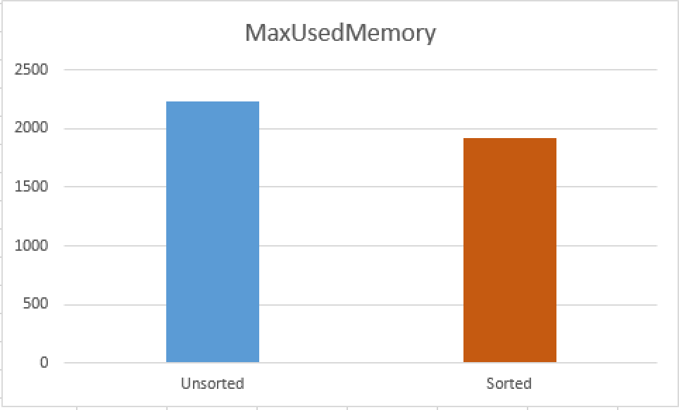 The difference between occupied memory is simply around 15%, which is very significant when we are talking about structures as L-Caches – any miss on the L2 cache is payed very dearly since the difference of latencies between L2 & L3 are significant (to my knowledge it is around 4 times slower plus do not forget that L3 is already a shared cache so in the future once Microsoft makes Batch Mode NUMA-aware the difference might be even bigger).
Overall the difference in performance might be very significant whenever doing Column Clustering on the most common column that you have in your workload, and not only because of the Segment Elimination but because of the applied compression and Late Materialisation.
to be continued with Clustered Columnstore Indexes – part 43 (“Transaction Log Basics”)