Continuation from the previous 39 parts, starting from https://www.nikoport.com/2013/07/05/clustered-columnstore-indexes-part-1-intro/
It’s time to take a look into the algorithms that Microsoft is using to compress Columnstore Indexes. I have presenting on this topic for quite some time and especially during Workshops I use to spend some time showing them and so today I am transferring this knowledge into my blog.
There are 3 basic phases for the Columnstore Index creation:
- Row Groups Separation
- Segment Creation
- Compression
This blog post is focused on the 3rd phase – Compression.
There are a number of compression technics that are being applied for achieving the best possible compression while not spending way too much CPU, and those that I know about are the following ones:
- Value Scale
- Bit Array
- Run-length Encoding
- Dictionary encoding
- Huffman encoding
- Lempel-Ziv-Welch
- Binary compression
Important: Before advancing with compression, SQL Server samples statistics with one of the algorithm as described in the 3rd blog post (More Internals). The amount of data that is being sampled is being chosen between 1% or 1 Million Rows, whichever has been reached first.
Value Scale
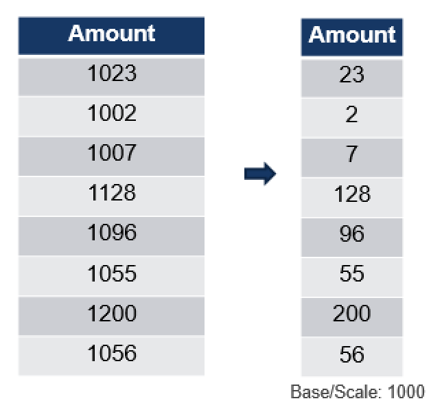 Value scale is a very basic principle, which is based on the some arithmetic operation (addition/multiplication/division/etc) that is applied commonly to all values inside compressed column. In my example you can see that the column contains the following values: 1023, 1002, 1007 … having a common part that all of them are starting with 1000, and so we can use value 1000 as a Value Scale applying multiplication to all of our values and storing just the right part of the equation.
You might ask – what kind of difference it will make in this case ? Well, to store a value such as 1023 in SQL Server you will need at least 2 bytes, while for any values between 0 and 255, you will be able to use just 1 byte. This means that storing values in this way decreases the storage space needed 50%!
The information on the Value Scale can be freely found by consulting sys.column_store_segments DMV, where it is shown in the base_id column.
Bit Array
Bit Array is a data structure that allows to store certain types of information compactly – thus compressing it.
This type of compression works well when we have a few distinct values stored in our column, because this algorithm stores a bit column for each of the distinct values found in the compressed structure (Segment).
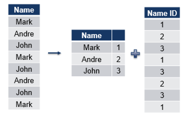
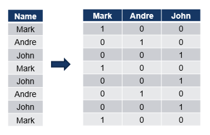 In this example we have a single column with 3 distinct values as well as 8 total values. On the right side you can see that we create a bit column with possible values of 0 & 1 and 3 columns with all those distinct values that could be found in the original column.
This way if we issue a query with a single predicate, such as:
select name from dbo.T where name = 'Niko';
we do not even have to scan our table, it is enough to read the meta-information to identify that Niko is the name that is not present in the values of our column and hence SQL Server does not need to make any reads from the table.
If we issue a different statement
select name from dbo.T where name = 'Andre';
we can easily join the resulting bit mask with our column in order to identify the values that we are looking for.
In the case of multiple predicates, such as
select name from dbo.T where name in ('Andre', 'John');
we can join the Bitmap mask of both columns in order to create the final vector that shall be applied with our source Rows.
Note that this is very same way that the Deleted Bitmap is functioning.
This algorithm is well suited for parallelism – imagine we have 256 distinct values in a Segment and 2 cores – we can give each of the cores 16 bytes to analyse and process.
Run-Length Encoding
Run-Length Encoding is very simple type of compression which effectiveness is proportional to the number of distinct values, such as Bit Array.
After sampling the data compression algorithm tries to sort the data on different columns in order to make a crucial decision on which column sorting shall bring the best results for the compression. For each new value found, we store it inside the hash dictionary and for each consecutive repetition we simply increase the number of the value stored in our hash table.
In this example we have a simple table with 2 columns – [Name] and [Last Name], and so we make 2 runs, trying to sort table rows on [Name] and compress them:
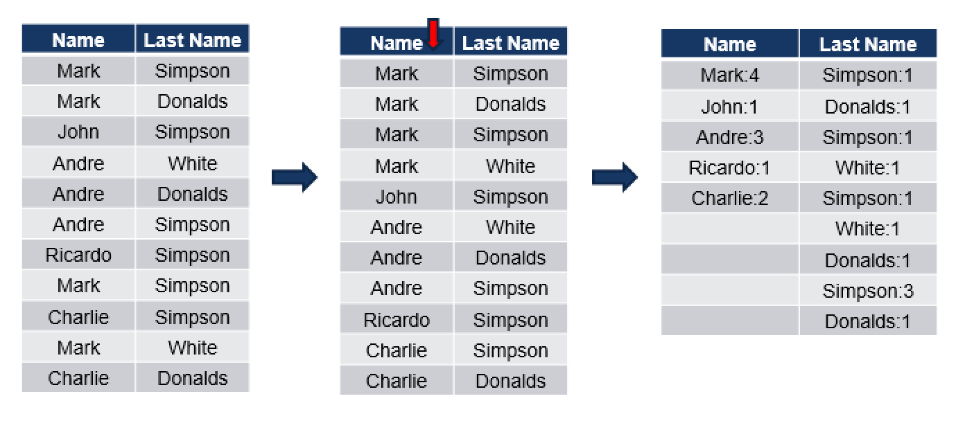 As you can see we have sorted data on the [Name] column in the first phase and in the second phase we parse through distinct values and store the number of times they can be found in our table.
The result of the 1st run is that we have 5 distinct values in our [Name] column and 9 values in our [Last Name] Column.
When accessing some value we simply add the number of times every value is found inside our column and so reach the right row. For example, if we are looking for the row number 8, we count that we have Mark 4 times, John 1 time, Andre 3 times and Ricardo 1 time – and so the first name of the person is Ricardo. If we do the same math on the [Last Name] column we shall find that the last name of the person for the Row number 8 is Simpson.
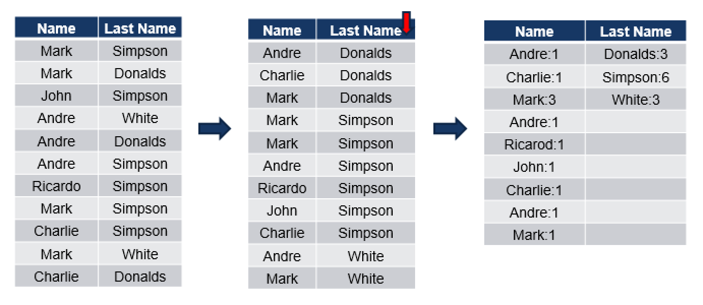 During the second run we sort on the [Last Name] column and here we have 9 values for the first name and 3 values for the Last Name. This seems to be a more effective compression method for the sampled data and so it will be used for compressing potentially.
Dictionary Encoding
 Dictionary Encoding is based on the principle of finding repetitive values (it is extremely effective with variable character type) and encoding them with smaller values, such as in example provided on the picture – I have simply given each of the strings inside my table some id, which occupies significantly less space, thus compressing the original information.
This is a fairly simple method, since there are a number of different methods, which are using advanced sampling and statistics in order to achieve the best compression possible.
In this compression method the size of my dictionary might be an issue to the performance and so the algorithm needs to balance its size, sometimes limiting it in order to avoid performance problems in other areas. So far I know, the size of the dictionary in Columnstore Indexes is varying from 56 bytes to 16 megabytes, and when the maximum size for a dictionary is reached – the maximum number of rows per Row Group shall be limited (aka dictionary pressure).
Huffman Encoding
Huffman Encoding is a fairly advanced form of Dictionary Encoding which is using variable-length code table, based on the estimation of frequency of appearance for each of the values, found in the source. After establishing these probability values (weights), a tree structure is created, assigning the most frequent values the fewer number of bits.
There is a fair number of Huffman Encoding variations, such as Adaptive, Length-limited, n-ary, Canonical, etc.
The actual used algorithm in the Columnstore Indexes is not publicly known at the moment.
Lempel-Ziv-Welch:
Lempel-Ziv-Welch algorithm might be the most used compression algorithm in the IT, being used from Unix compress command to never-disappearing GIF format. If you are interested in the details, please consult the link to Wikipedia article.
Binary Compression
After one or multiple compression algorithms have been applied we are compressing data by using the super-secret xVelocity compression into a LOB, storing at our disk. The LOB itself is not a simple large binary object, because it has types and subtypes and so I guess the xVelocity is doing some adaptations when recognising different patterns.
One important exception to the above written rule is the Columnstore Archival compression, which is basically adding a new layer of compression by using a modified and optimised LZ77 compression.
Almost real-life example:
To show some real data inside the compressed columnstore, I will use the famous & unsupported DBCC CSIndex command on my favourite database – ContosoRetailDW:
Lets restore our Database, drop all Primary & Foreign Keys from the Fact Tables and create a Clustered Columnstore on the dbo.FactOnlineSales table:
USE [master]

ALTER DATABASE [ContosoRetailDW] SET SINGLE_USER WITH ROLLBACK IMMEDIATE;

RESTORE DATABASE [ContosoRetailDW]
	FROM  DISK = N'C:\Install\ContosoRetailDW.bak' WITH  FILE = 1,
		MOVE N'ContosoRetailDW2.0' TO N'C:\Data\ContosoRetailDW.mdf',
		MOVE N'ContosoRetailDW2.0_log' TO N'C:\Data\ContosoRetailDW.ldf',
		NOUNLOAD,  STATS = 5;

ALTER DATABASE [ContosoRetailDW] SET MULTI_USER;

use ContosoRetailDW;

alter table dbo.[FactOnlineSales] DROP CONSTRAINT PK_FactOnlineSales_SalesKey
alter table dbo.[FactStrategyPlan] DROP CONSTRAINT PK_FactStrategyPlan_StrategyPlanKey
alter table dbo.[FactSales] DROP CONSTRAINT PK_FactSales_SalesKey
alter table dbo.[FactInventory] DROP CONSTRAINT PK_FactInventory_InventoryKey
alter table dbo.[FactSalesQuota] DROP CONSTRAINT PK_FactSalesQuota_SalesQuotaKey

alter table dbo.[FactOnlineSales] DROP CONSTRAINT FK_FactOnlineSales_DimCurrency
alter table dbo.[FactOnlineSales] DROP CONSTRAINT FK_FactOnlineSales_DimCustomer
alter table dbo.[FactOnlineSales] DROP CONSTRAINT FK_FactOnlineSales_DimDate
alter table dbo.[FactOnlineSales] DROP CONSTRAINT FK_FactOnlineSales_DimProduct
alter table dbo.[FactOnlineSales] DROP CONSTRAINT FK_FactOnlineSales_DimPromotion
alter table dbo.[FactOnlineSales] DROP CONSTRAINT FK_FactOnlineSales_DimStore
alter table dbo.[FactStrategyPlan] DROP CONSTRAINT FK_FactStrategyPlan_DimAccount
alter table dbo.[FactStrategyPlan] DROP CONSTRAINT FK_FactStrategyPlan_DimCurrency
alter table dbo.[FactStrategyPlan] DROP CONSTRAINT FK_FactStrategyPlan_DimDate
alter table dbo.[FactStrategyPlan] DROP CONSTRAINT FK_FactStrategyPlan_DimEntity
alter table dbo.[FactStrategyPlan] DROP CONSTRAINT FK_FactStrategyPlan_DimProductCategory
alter table dbo.[FactStrategyPlan] DROP CONSTRAINT FK_FactStrategyPlan_DimScenario
alter table dbo.[FactSales] DROP CONSTRAINT FK_FactSales_DimChannel
alter table dbo.[FactSales] DROP CONSTRAINT FK_FactSales_DimCurrency
alter table dbo.[FactSales] DROP CONSTRAINT FK_FactSales_DimDate
alter table dbo.[FactSales] DROP CONSTRAINT FK_FactSales_DimProduct
alter table dbo.[FactSales] DROP CONSTRAINT FK_FactSales_DimPromotion
alter table dbo.[FactSales] DROP CONSTRAINT FK_FactSales_DimStore
alter table dbo.[FactInventory] DROP CONSTRAINT FK_FactInventory_DimCurrency
alter table dbo.[FactInventory] DROP CONSTRAINT FK_FactInventory_DimDate
alter table dbo.[FactInventory] DROP CONSTRAINT FK_FactInventory_DimProduct
alter table dbo.[FactInventory] DROP CONSTRAINT FK_FactInventory_DimStore
alter table dbo.[FactSalesQuota] DROP CONSTRAINT FK_FactSalesQuota_DimChannel
alter table dbo.[FactSalesQuota] DROP CONSTRAINT FK_FactSalesQuota_DimCurrency
alter table dbo.[FactSalesQuota] DROP CONSTRAINT FK_FactSalesQuota_DimDate
alter table dbo.[FactSalesQuota] DROP CONSTRAINT FK_FactSalesQuota_DimProduct
alter table dbo.[FactSalesQuota] DROP CONSTRAINT FK_FactSalesQuota_DimScenario
alter table dbo.[FactSalesQuota] DROP CONSTRAINT FK_FactSalesQuota_DimStore;
GO

Create Clustered Columnstore index PK_FactSales
    on dbo.FactSales;
Now we need to determine the key parameters (HOBT_ID and DB_ID) for later usage:
select top 1 seg.hobt_id, DB_ID()
    from sys.column_store_segments seg
	inner join sys.partitions as p
		ON seg.partition_id = p.partition_id
	where OBJECT_id = OBJECT_ID('FactOnlineSales');
In my current case the ID of the HOBT was 72057594049069056 and the Database ID was equal to 7.
Now let’s run a DBCC CSIndex in order to see the contents of the Dictionary for the SalesOrderNumber column:
dbcc traceon (3604);
GO

dbcc csindex (
    7,
    72057594049069056,
    8, /*SalesOrderNumber*/
    0, /*Segment*/
    2, /*Dictionary*/
    0
);
 I want you to look with more attention not at the header, but at the HashTable Array Data, and more specifically at the values stored for each of the Indexes. Let’s take the very first value from it – 8732 and check if we can find in the original table by using the following query:
select top 20 SalesOrderNumber, OnlineSalesKey, StoreKey
	from dbo.FactOnlineSales
	where SalesOrderNumber like '%8732%';
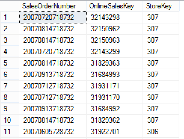 I can easily see where those values are coming from – each of my returned rows ends with 8732, and so it is easy to understand that compression algorithm has chosen a substring out of our nvarchar field to compress, most probably basing on its frequency of appearance in the destination table and respective segment. In practice running Count(*) on the table with the same predicate returns a fairly interesting number of 462.
Now you have some start information as well as the weapon for discovering more – Happy Discovering!
to be continued with Clustered Columnstore Indexes – part 41 (“Statistics”)