This is the 6th blog post in the growing series of blogpost on the Graph features within SQL Server and Azure SQL Database that started at SQL Graph, part I.
This time I want to focus on one of the most important measures that there are out there – the Closeness Centrality.
There are a number of different measures that are very common for the Graph applications with the likes of Closeness Centrality, Betweenness Centrality, Eigenvector etc, each one with different application scenarios and importance o and in the next blog posts I will be going through some of them. Notice that from my personal experience a number of times, the application of these measures is often mixed together in order to view the different angles of the centrality.
But not willing to jump ahead too much, let’s focus right now only on the Closeness Centrality.
Closeness Centrality
The real center of the network or also known as The King of the Network, Closeness Centrality is a measure which represents the relative location of the Vertice to the center of the network, or better to say the average distance to all other Vertices within that network.
This measure results in the high effectiveness of information spreading/flow within the given network, because of the necessary number of Edges to cross to reach to any given connected Vertice.
The application areas of the Closeness Centrality is high, starting with the organisational structure analysis and diving into the social networks (who is the real king, since you might not need to have the highest number of edges (aka followers) to be a significant influencer – you will need to have the right ones), computer networks & telecommunications (estimation of the speed for information spreading), bioinformatics and many more.
The calculation of the Closeness Centrality consists of the relatively simple formula:
Closeness Centrality = (The_Number_Of_Vertices – 1) / SUM (Shortest_Paths_To_All_Vertices)
where a huge and extremely important assumption is to have some connected vertices, otherwise it won’t make any sense. :)
If you look into some of the scientific papers or some of the other database produced solutions, there will be some variations of the types of the Closeness Centrality, how to calculate it and the best algorithm on calculating it with the highest efficiency. I am consciously ignoring the raw, the normalised, the disconnected and similar more complex scenarios, since I want to keep this blog post more accessible for those who are new to the graph databases.
With the release of the Shortest Path function in SQL Server 2019 CTP 3.0, the entry barrier for this type of calculations has been suddenly lifted and there is virtually no excuse in order not to start analysing your networks within Azure SQL Database & SQL Server 2019 (trying in CTP’s and get ahead with the expected release … I would guess somewhere around the MS Ignite in early November :))
We won’t be able to do the weighted calculations right now, because in the upcoming release of the SQL Server 2019 the focus of the implementation will be to support non-weighted networks, but do not get totally disappointed right away since there are so many incredibly interesting things that we can do with the current system and providing a valuable feedback and starting to apply this feature will be the key to show that the weighted calculations are really needed by the market.
A practical example of Closeness Centrality
Here is a definition of a simple graph with just 6 nodes, that can be seen in the matrix below:
| Alpha Beta | Max Max | John Doe | Master Blaster | Felix Fixit | Trim Trimell | |
| Alpha Beta | – | 1 | 0 | 0 | 0 | 0 |
| Max Max | 1 | – | 1 | 0 | 0 | 0 |
| John Doe | 0 | 1 | – | 1 | 1 | 0 |
| Master Blaster | 0 | 0 | 1 | – | 1 | 0 |
| Felix Fixit | 0 | 0 | 1 | 1 | – | 1 |
| Trim Trimell | 0 | 0 | 0 | 0 | 1 | – |
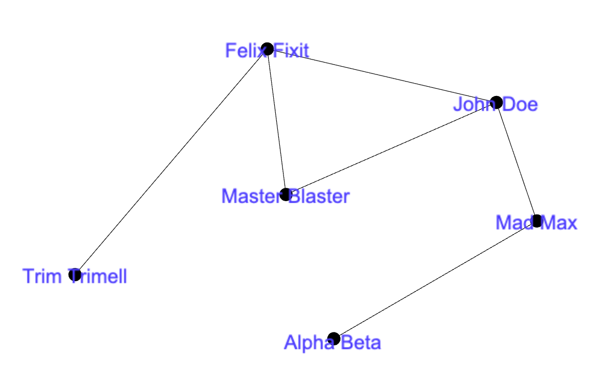 On the left side of this text you can see the visual representation of the defined graph where you can make your educated guesses on which node will be the Queen/King of our network. The network itself is extremely simple and a human eye should be able to help to do this type of calculations in a network with a very small diameter, but make no mistake – once we are going into hundreds and thousands of Vertices, the task will become unbearable and precisely in these cases the SQLGraph will become our good friend very fast.
Let us calculate the shortest path values for the “Alpha Beta” Vertice, resulting in the following results:
- Mad Max: 1
- John Doe: 2
- Master Blaster: 3
- Felix Fixit: 3
- Trim Trimell: 4
This is exactly the number of hopes through the edges that we need to do in order to reach the respective vertice.
Now, in our formula we shall simply need to make a sum of all those values -> 1 + 2 + 3 + 3 + 4 = 13 and divide it through the number of the vertices, minus 1 because we do not need to calculate the path to the starting vertice “Alpha Beta” itself -> 6 – 1 = 5.
The Closeness Centrality for the Vertice “Alpha Beta” is hence 5 / 13 = 0.384615
Let’s do the same exercise of calculating the shortest paths for the Vertice “John Doe”:
- Alpha Beta: 2
- Mad Max: 1
- Master Blaster: 1
- Felix Fixit: 1
- Trim Trimell: 2
The resulting sum of the shortest paths for this vertice shall be 2 + 1 + 1 + 1 + 2 = 7, and given the number of vertices to use in the division is the same good old 5, the final result for the Closeness Centrality for the Vertice “John Doe” shall be 5 / 7 = 0.714286!
The calculated shortest paths between each of the nodes is to be found in the table below, in order to simplify the understanding:
| Alpha Beta | Max Max | John Doe | Master Blaster | Felix Fixit | Trim Trimell | CLOSENESS CENTRALITY | |
| Alpha Beta | – | 1 | 2 | 3 | 3 | 4 | 5 / (1+2+3+3+4) = 0.384615 |
| Max Max | 1 | – | 1 | 2 | 2 | 3 | 5 / (1+1+2+2+3) = 0.555556 |
| John Doe | 2 | 1 | – | 1 | 1 | 2 | 5 / (2+1+1+1+2) = 0.714286 |
| Master Blaster | 3 | 2 | 1 | – | 1 | 2 | 5 / (3+2+1+1+2) = 0.555556 |
| Felix Fixit | 3 | 2 | 1 | 1 | – | 1 | 5 / (3+2+1+1+1) = 0.625000 |
| Trim Trimell | 4 | 3 | 2 | 2 | 1 | – | 5 / (4+3+2+2+1) = 2.4 |
Having the higher number of the Closeness Centrality makes you closer to the center of the network/graph and thus the results for our tiny graph are following, ordered by the closeness to the center:
- John Doe: 0.714286
- Felix Fixit: 0.625000
- Master Blaster: 0.555556
- Mad Max: 0.555556
- Trim Trimell: 0.416667
- Alpha Beta: 0.384615
and where our Queen/King of the network is the Vertice “John Doe”.
Practical Closeness Centrality in Sql Server
For the practical test let us set up the very same tables as in the previous post/exercise – Person (Node) & Follows (Edge), this time making sure that every single connection is reciprocated:
DROP TABLE IF EXISTS dbo.Follows;
DROP TABLE IF EXISTS dbo.Person;

CREATE TABLE dbo.Person(
	PersonID BIGINT IDENTITY(1,1) NOT NULL PRIMARY KEY CLUSTERED ,
	FULLNAME NVARCHAR(250) NOT NULL ) AS NODE;

CREATE TABLE dbo.Follows(
    Since DATETIME2 NULL,
    CONSTRAINT EDG_Person_Follows CONNECTION (Person TO Person)
)
AS EDGE;
and now the data and the connection definitions:
TRUNCATE TABLE dbo.Follows;
DELETE FROM dbo.Person;

INSERT INTO dbo.Person
	VALUES ('John Doe'),
		   ('Alpha Beta'),
			('Mad Max'),
			('Master Blaster'),
			('Felix Fixit'),
			('Trim Trimell');


-- Everyone whos name starts with letters C & M follows John Doe
INSERT INTO dbo.Follows
	SELECT	p1.$node_id as from_obj_id,
			pf.to_obj_id,
			GetDate()
		FROM dbo.Person p1
			CROSS APPLY (SELECT p2.$node_id as to_obj_id FROM dbo.Person p2 WHERE p2.PersonId <> p1.PersonId and p2.Fullname = 'Mad Max') pf
		WHERE (p1.FULLNAME = 'Alpha Beta')

-- Mad Max follows John Doe & Alpha Beta
INSERT INTO dbo.Follows
SELECT	p1.$node_id as from_obj_id,
			pf.to_obj_id,
			GetDate()
		FROM dbo.Person p1
			CROSS APPLY (SELECT p2.$node_id as to_obj_id FROM dbo.Person p2 WHERE p2.PersonId <> p1.PersonId and (p2.FULLNAME = 'John Doe' OR p2.FULLNAME = 'Alpha Beta')) pf
		WHERE p1.FULLNAME = 'Mad Max';

-- John Doe follows Master Blaster, Mad Max & Felix Fixit
INSERT INTO dbo.Follows
SELECT	p1.$node_id as from_obj_id,
			pf.to_obj_id,
			GetDate()
		FROM dbo.Person p1
			CROSS APPLY (SELECT p2.$node_id as to_obj_id FROM dbo.Person p2 WHERE p2.PersonId <> p1.PersonId and (p2.FULLNAME IN  ('Mad Max', 'Master Blaster', 'Felix Fixit'))) pf
		WHERE p1.FULLNAME = 'John Doe';

-- Master Blaster follows John Doe & Felix Fixit
INSERT INTO dbo.Follows
SELECT	p1.$node_id as from_obj_id,
			pf.to_obj_id,
			GetDate()
		FROM dbo.Person p1
			CROSS APPLY (SELECT p2.$node_id as to_obj_id FROM dbo.Person p2 WHERE p2.PersonId <> p1.PersonId and (p2.FULLNAME IN  ('John Doe', 'Felix Fixit'))) pf
		WHERE p1.FULLNAME = 'Master Blaster';

-- Felix Fixit follows Master Blaster, John Doe & Trim Trimell
INSERT INTO dbo.Follows
SELECT	p1.$node_id as from_obj_id,
			pf.to_obj_id,
			GetDate()
		FROM dbo.Person p1
			CROSS APPLY (SELECT p2.$node_id as to_obj_id FROM dbo.Person p2 WHERE p2.PersonId <> p1.PersonId and (p2.FULLNAME IN  ('Master Blaster', 'John Doe', 'Trim Trimell'))) pf
		WHERE p1.FULLNAME = 'Felix Fixit';

-- Trim Trimell follows Felix Fixit
INSERT INTO dbo.Follows
SELECT	p1.$node_id as from_obj_id,
			pf.to_obj_id,
			GetDate()
		FROM dbo.Person p1
			CROSS APPLY (SELECT p2.$node_id as to_obj_id FROM dbo.Person p2 WHERE p2.PersonId <> p1.PersonId and (p2.FULLNAME IN  ('Felix Fixit'))) pf
		WHERE p1.FULLNAME = 'Trim Trimell';
We are ready for the awesomeness of the SQL Graph and so let’s write a query to calculate the Closeness Centrality.
using the basis from the previous post in the series and in the first step let us list all the existing connections between all Vertices in our graph:
SELECT
	p1.PersonId,
	p1.FULLNAME as StartNode,
	LAST_VALUE(p2.FULLNAME) WITHIN GROUP (GRAPH PATH) AS FinalNode,
	COUNT(p2.PersonId)  WITHIN GROUP (GRAPH PATH) AS Levels
FROM
	dbo.Person p1,
	dbo.Person FOR PATH p2,
	dbo.Follows FOR PATH follows
WHERE
	MATCH(
		SHORTEST_PATH(p1(-(follows)->p2)+)
	);
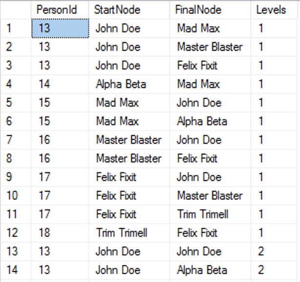 And as you can see on the left side, the list with a part of the 36 results that we have received in return. This is a very easy stuff to write, once you understand how to work with the SHORTEST_PATH. The function SHORTEST_PATH is applied within the MATCH clause which itself is a search predicate for our query. If you are interested in the details, please consider visiting SQL Graph, part V – Shortest Path.
Now all we have to do is to wrap an additional query around this list of the shortest paths, group it by origin Vertice (StartNode) and calculate the sum of the Levels (Edges we have to cross to reach the final node) and order the results by descending values of the calculated Closeness Centrality, and using this value to divide the number of Vertices – 1 by the result of our calculations e voilá:
SELECT StartNode, CAST( (SELECT COUNT(*) - 1 FROM dbo.Person)  / CAST(SUM(Levels) AS DECIMAL(9,0)) as DECIMAL(9,6)) as ClosenessCentrality
	FROM (
		SELECT
			p1.PersonId,
			p1.FULLNAME as StartNode,
			LAST_VALUE(p2.FULLNAME) WITHIN GROUP (GRAPH PATH) AS FinalNode,
			COUNT(p2.PersonId)  WITHIN GROUP (GRAPH PATH) AS Levels
		FROM
			dbo.Person p1,
			dbo.Person FOR PATH p2,
			dbo.Follows FOR PATH follows
		WHERE
			MATCH(
				SHORTEST_PATH(p1(-(follows)->p2)+)
			)
		) src
	WHERE StartNode <> FinalNode
	GROUP BY StartNode
	ORDER BY ClosenessCentrality DESC;
 Pretty amazing how easy and how fast we can get the detailed results, for which should we need to scale up – all we need to do is to apply the very same query without any further modifications and this is incredibly awesome.
Important Notes
I want to repeat myself and reforce that I did not considered more complex scenarios, such as when we do not have a reciprocal connection back between the Vertices and when we have disconnected Vertices in our graph. Stay tuned because this series will definitely be focusing on those scenarios.
Final Notes
I love that the whole class of the graph solutions became available to everyone to apply. Without pulling the data out of your secure relational platform, you can do pretty amazing things, which WITHOUT MAJOR EFFORT were reserved for those who had access to the graph databases.
Yes, we could do any possible solution in Sql Server before, but the performance was slow and the ease of the development was non-existing – not many people would be able to support real-world complex scenarios.
I am impatiently waiting for more developments and support for even more functions – enabling the Sql Server developers to do some incredible stuff. :)
to be continued …
Niko,
Wrong number:
Trim Trimell 4 3 2 2 1 – 5 / (4+3+2+2+1) = 2.4
Should be 0.416667
Hi Vlad,
I just checked the article and it contains exactly those numbers or do I see something wrong here?
Best regards,
Niko
Excellent article, was wondering if you found a way to filter on the edge table when using shortest_path ? Only way I have found so far is using a view on the edge table.
Hi Nojetlag,
can you provide a concrete example so that I would be able to understand better the difficulty.
Thank you.
Best regards,
Niko
Hi Niko,
thanks for your excelent articles to graphs.
Do you have any information what will come with the next version of SQL-Server and how the next version will be available?
Hi Martin,
There is no such information publicly available.
What I honestly expect are just a few smaller functionalities, rather than big investment. Unfortunately.
Best regards,
Niko
Hi Nojetlag,
i found a way to limit the edges that are used. In this statement I limit to the ones that only follows since the last five days.
SELECT StartNode, CAST( (SELECT COUNT(*) – 1 FROM dbo.Person) / CAST(SUM(Levels) AS DECIMAL(9,0)) as DECIMAL(9,6)) as ClosenessCentrality
FROM (
SELECT
p1.PersonId,
p1.FULLNAME as StartNode,
LAST_VALUE(p2.FULLNAME) WITHIN GROUP (GRAPH PATH) AS FinalNode,
COUNT(p2.PersonId) WITHIN GROUP (GRAPH PATH) AS Levels
FROM
dbo.Person p1,
dbo.Person FOR PATH p2,
(SELECT * FROM dbo.Follows WHERE Since > (GetNow() – 5))FOR PATH follows
WHERE
MATCH(
SHORTEST_PATH(p1(-(follows)->p2)+)
)
) src
WHERE StartNode FinalNode
GROUP BY StartNode
ORDER BY ClosenessCentrality DESC;